WAVEFORMS ASSOCIATED WITH ASTABLE MULTIVIBRATOR

EDITOR: B. SOMANATHAN NAIR

1. INTRODUCTION

In the previous blog, we had seen how an astable multivibrator works. In this blog, we discuss the waveforms associated with astable multi. We must show that the circuit produces square waves.

2. WAVEFORMS GENERATED AT VARIOUS TERMINALS

Figures 1 and 2 show the waveforms at the collector and base, respectively, of transistor T₁. Similarly Figs. 3 and 4 show the waveforms at the collector and base, respectively, of transistor T₂.

            Consider the instant t₀ at which we assume that T₁ has just turned-off and T₂ has just turned-on. At this instant, we find that collector voltage V_CE2 of T₂ drops from V_CC (=10 V) to V_CESAT (= 0.2 V). Correspondingly, base voltage V_BE1 of T₁ drops from V_BESAT (= 0.8 V) by the same amount V_CC−V_CESAT (= 9.2 V). In effect, from the figure, we find that V_BE1 drops to a voltage equal to [V_BESAT − (V_CC−V_CESAT) = 0.8 −(10−0.2)= −9 V]. Thus V_BE1 drops from a small positive value of +0.8 V to a large negative value of −9 V at the instant of transition.

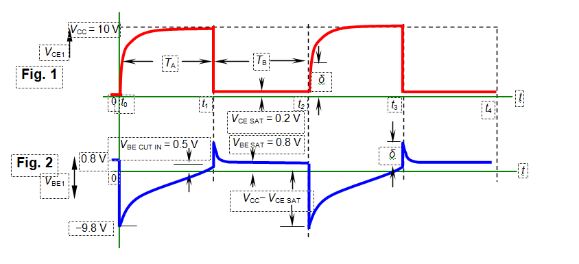
        We also notice that at instant t₀, V_CE1 rises from V_CESAT at first by a sudden jump of δ volts (δ can be calculated using an equivalent circuit, which will be done in anther blog) and then by an exponential rise to V_CC. At the same time, we notice that V_BE2 jumps up by the same amount of δ volts from V_BECUT-IN (= 0.5 V). Once V_BE2 jumps above V_BESAT (= 0.8 V), saturation sets in. This reduces V_BE2 back to V_BESAT exponentially. It will then remain constant at this value until the next switching of transistors occurs at instant t₁. 

            Let us now consider the interval (t₁ – t₀). In this interval, we observe that V_BE1 rises from [V_BESAT – (V_CC – V_CESAT)] exponentially to V_BECUT-IN (= 0.5 V), at time t = t₁. This turns T₂ into the ON state and T₁ into the OFF state. As discussed earlier, this sudden turn-on of T₂ draws a small initial collector current I_C2, which increases the drop V_RC2 and reduces V_CE2 (and hence V_BE1). This decrease in V_BE1 is reflected by the large drop in the collector current of T₁, I_C1. The large drop in I_C1 is due to the amplification by T₁. A similar amplification by T₂ brings about the desired transitions (turning-on of T₂ and turning-off of T₁). These sudden transitions give rise to the transients found in the waveforms shown in Figs. 1 to 4.

3. FREQUENCY OF OSCILLATION    

To obtain an expression for the free-running frequency (or frequency of oscillation), we make use of the basic capacitance-charging equation

                                                                                                            

v_C = V_F ‒ (V_F‒ V_I) exp(‒t/RC)  (1)  

where v_C is the voltage across the capacitor, V_I is the initial voltage from which the capacitor starts charging, and V_F is the final voltage to which the capacitor gets charged to. From Figs. 3 and 4, we find that V_I = V_BESAT − (V_CC−V_CESAT), v_C= V_BECUT-IN, and V_F = V_CC. We also notice that R = R_B.  Substituting these values in Eq. (1), we get

         

V_BECUT-IN =V_CC ‒  [V_CC ‒ (V_BESAT − V_CC+V_CESAT)] exp(‒t/RC)        

                                = V_CC ‒  [2V_CC ‒ (V_BESAT +V_CESAT)] (2)

                                                                                                                            

Rearranging Eq. (2) yields                               

    exp(‒t/R_BC) = [2V_CC ‒ (V_BESAT +V_CESAT)]/(V_CC ‒ V_BECUT-IN)  (3)

                                                                                                           

From Eq. (3) we get the expression for the half-period of oscillation T_A as

                                                                                   

                        T_A = R_BC ln {[2V_CC ‒ (V_BESAT +V_CESAT)]/(V_CC ‒ V_BECUT-IN)} (4)

If V_BECUT-IN, V_BESAT, and V_CESAT are negligible compared to V_CC, Eq. (4) reduces to

         T_A = R_BC ln (2V_CC/V_CC) = R_BC ln 2 = 0.69 R_BC  (5)

                                               

In a similar way, we find for symmetrical waveform

          T_B = R_BC ln (2V_CC/V_CC) = R_BC ln 2 = 0.69 R_BC  (6)

                                                                          

Thus the total period of oscillation is

 

     T­ = T_B + T_A= 1.38 R_BC    (7)                              

                                                                                                                

And the frequency of oscillation for symmetrical operation

  f_o =1/T = 1/ 1.38 R_BC    (8)