BLOCK DIAGRAM REDUCTION IN CONTROL SYSTEMS - A SIMPLE ALGEBRAIC METHOD

B. SOMANATHAN NAIR

P. S. CHANDRAMOHANAN NAIR

ABSTRACT

In this paper, we present a very simple and straightforward method for reducing complex-looking block diagrams. The main advantage of this method is that the last step in the reduction process directly gives the expression of the transfer function of the system. The reduction process requires only an introductory knowledge of elementary algebra.

1. INTRODUCTION

         Currently two methods are described in the Control-System literature^1,2,3,4 for reducing complex-looking block diagrams. These are, respectively, the ‘Mason’s gain formula’ and the ‘moving-block method’.

            Mason’s gain formula^1,2,3 suffers from the following drawbacks:

^·       It becomes difficult in some cases to identify all the feed-forward and feed-back paths.

^·    In several cases, it may become difficult to identify all the closed loops in the system. It is interesting to note that the number of closed loops in Problem 3.14 of Reference 1 is actually 4; but it was miscalculated as 3 loops in the Reference 2 (this was corrected in Reference 1). This proves our argument.

^·     It is difficult for a beginner to identify all the touching and non-touching loops in the system.

^·      Identification of co-factors is difficult in many situations.

The difficulties mentioned above will lead to a wrong derivation of the control ratio of the system.

           The second method known as 'moving-block (or summing-point)' method^1,2 is also a complicated operation. The problems associated with this method are the following:

·        It is difficult to remember several expressions related to the moving of a block in the forward direction and in the reverse direction past a summing point.

·     For each such movement, one has to redraw the new block-diagram configuration.

·    Unless the above operations are carefully done, this method can also lead to wrong answers.

            The method described in this paper involves no previous knowledge of any complex formulas and requires only an elementary knowledge of algebra. The method is simple, straightforward and can be applied easily.

2. A NEW SIMPLE ALGEBRAIC METHOD

The first step in the new method is to identify and name all the nodes in the block as E₁,  E₂, etc., where E’s represent respective error signals. Once the nodes are named, we start writing simple algebraic equation for each node that gives the value of the E signal of that node. The method can be best illustrated by explaining an actual example.

Example 1: Figure 1 shows the block diagram to be reduced and Fig. 2 shows the same block diagram with the respective nodes designated.

            In Fig. 2, we find that there are six nodes, designated as E₁, E₂, E₃, E₄,  E₅, and E₆, respectively. Of these six, we immediately recognize that node 

E₅ = C

            We now proceed to write the algebraic equation for each of the nodes. Thus at Node 1, we find

           

                                                         E₁ = R ‒ C                                          (1)

At Node 2, the equation becomes

                                     

                                                       E₂ = E₁ + E₅ H₁                                    (2)

Now, in our method, we immediately substitute for E₁ from Eq. (1) into Eq. (2). Thus

                                   

                                                   E₂ = R ‒ C + E₅H₁                                    (3)

At Node 3, the equation is

   

                                                                 E₃ = G₁H₂                                   (4)

We now substitute for E₂ from Eq. (3) into Eq. (4). Thus

                                   

        E₃ = G₁(R ‒ C + E₅H₁)

                                                = G₁R ‒ G₁C + E₅G₁H₁       (5)

Now, the equation at Node 4 is

                                           E₄ = E₃ ‒ C H₂                                 (6)

                                                                                         

Substituting for E₃ from Eq. (5) into Eq. (6) yields

                       

                              E₄ = G₁R ‒ G₁C + E₅G₁H₁ ‒ C H₂                                         (7)

Next we have the equation for Node 5 as

                                                   E₅ = E₄G                                   (8)

Now, substituting for E₄ from Eq. (7) into Eq. (8), we get

                               E₅ = (G₁R ‒ G₁C + E₅G₁H₁ ‒ C H₂)G₂                                                               

   =G₁G₂R‒G₁G₂C+E₅G₁G₂H₁‒CG₂                              (9)

Rearranging Eq. (9), we obtain

                                                E₅(1‒G₁G₂H₁)=G₁G₂R‒G₁G₂C‒CG₂H₂      (10)

from which we get

         E₅=G₁G₂R‒G₁G₂C‒CG₂H₂ /(1‒G₁G₂H₁)          (11)

Finally at the output node, we find

                                            C = E₆ = E₅G₃                                                             (12)

Substituting for E₅ from Eq. (11) into Eq. (12), and simplifying after manipulations, we get the control ratio

In the method described above, we have used the technique of substituting for each of the E functions from its previous equation. Thus equation for E₂ is obtained by substituting the expression for E₁, equation for E₃ is obtained by substituting the expression for E₂, and so on, until we reach the expression for C. This reduces the complexity of solving for all the equations simultaneously in the end, and greatly simplifies the solution. As can be seen from the procedure, the solution of the last equation yields the control ratio C/R directly.

Example 2: Figure 3 shows the block diagram of a system slightly more complex than the one shown in Fig. 1. In this case also, we proceed in the same manner as was done in the case of Example 1.

            In the diagram shown in Fig. 3, we first mark all the E (error) nodes. In this case we find that there are seven nodes. We also find that Node E₇ is output node C itself.

We now proceed to write the algebraic equation for each of the nodes. Thus at Node 1, we find

                                                     E₁ = R  ‒ E₄ H₁                                                               (1)

At Node 2, the equation is

                                               

                                                     E₂ = G₁ E₁                                                                         (2)

Now, we substitute for E₁ from Eq. (1) into Eq. (2), which yields

                                                

                                                 E₂ = RG₁ ‒ E₄ G₁ H₁                                                            (3)

 At Node 3, the relation becomes

                                                  E₃ = E₂ + E₆ H₃                                                            (4)

Substituting for E₂ from Eq. (3) into Eq. (4) gives

                                       E₃ = RG₁ ‒ E₄ G₁ H₁     + E₆ H₃                                                     (5)

The equation for Node 4 can be written as

                                                    

E₄ = E₃ G₂ = RG₁ G₂ ‒ E₄ G₁ G₂ H₁   + E₆ G₂ H₃                             (6)

where we have used Eq. (5). Rearranging Eq. (6), we get

                                                   E₄(1‒ G₁ G₂ H₁) =  RG₁ G₂  + E₆ G₂ H₃                       (7)

From Eq. (7), we find

    

                                                E₄=  (RG₁ G₂ + E₆ G₂ H₃ )  /(1‒ G₁ G₂ H₁)                       (8)

The equation for Node 5 is given by

E₅  = E₄‒ CH₂  = (RG₁ G₂ + E₆ G₂ H₃ )  /(1‒ G₁ G₂ H₁) ‒ CH₂                               (9)

where we have substituted for E₄ from Eq. (8) to yield E₅. Now, equation for Node 6 is

                                                      E₆ = G₃E                                                                 (10)

Substituting for E₅ from Eq. (9) into Eq. (10) gives the expression

                 

                                       

            E₆ =  (RG₁ G₂ + E₆ G₂ H₃ )G₃  /(1‒ G₁ G₂ H₁) ‒ G₃CH₂                          (11)

Rearranging Eq. (11), we have

                       

            E₆ (1‒ (H₃G₂G₃)/(1 + G₁G₂ H₁ )

                                   = RG₁G₂ G₃/[(1 + G₁G₂                                              (12)                              

At Node 7, the output C can now be written as

                                                            C = E₇ = E₆ G_{4                                                            ­}(14)

Substituting for E₆ from Eq. (13) into Eq. (14), we obtain

Rearranging Eq. (15), we find

From Eq. (16), we get the control ratio as

Example 3: Figure 4 shows a two-input control system. We have to obtain the control ratios C/R and C/D of this system.

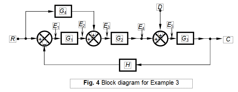
As in the above cases, we start with Node 1. With respect to Node 1, we find

                                                            R ‒ CH = E_{1                                                                   ­}(1)

At Node 2, we have

           

E₂ = G₁E₁ = (R ‒ CH)G₁                                                                (2)

Now, with respect to Node 3, we obtain

E₃ = E₂+ G₄R = (G₁+G₄)R ‒ CHG₁                                            (3)

At Node 4, we find

                       

E₄ = E₃G₂ = (G₁+G₄)R G₂ ‒ CHG₁G₂                                                  (4)

And at Node 5,

                                    E₅ = E_{4 ­}+ D = (G₁+G₄)R G₂ ‒ CHG₁G₂ +D                                  (5)

Finally, at Node 6,

C= G₃ E₅ = (G₁+G₄)R G₂G₃ ‒ CHG₁G₂ G₃  +D G₃                                                 (6)

Rearranging Eq. (6) yields the value of C [see  Eq. (7) below]

                                                                                                                                    (7)

            

To find C/R, we must assume D = 0. Then from Eq. (7), we obtain

        

 Similarly, to find C/R, we must assume R = 0. Then from Eq. (7), we obtain

3. CONCLUSION

We have demonstrated here a very simple and easy method for finding the control ratio of complex block diagrams representing control-system installations. It assumes no previous knowledge of finding feed-forward or feed-back paths and other complex computations involved in the usage of Mason’s gain formula nor does it require the remembrance of any complicated block-moving formulas. All it requires is the usage of simple algebra to solve the basic equation associated with each node of the system in a systematic and step-by-step fashion.

4. REFERENCES

1. Katsuhiko Ogata, Modern Control Engineering, 3^rd ed, Prentice-Hall, 1990
2. Katsuhiko Ogata, Modern Control Engineering, 2^rd ed, Prentice-Hall, 1997
3. Norman S. Nise,  Control Systems Engineering, 6^th ed., Wiley India, 2011
4. C. Mei, On Teaching the Simplification of Block Diagrams, Int. J. of Engng. Ed, (Great Britain) Vol. 18, No. 6, pp 697-703, 2002.

At Node 7, the output C can now be written as