BUTTERWORTH ANALOG FILTER DESIGN (CONTINUED)

EDITOR: B. SOMANATHAN NAIR

4. NUMERICAL DESIGN EXAMPLE

In the previous blog, we had given the procedure for designing an analog low-pass filter of the Butterworth type. In this blog, we give a practical numerical example of the design.

Example:  Design a Butterworth low-pass filter for the following specifications:

1.      Pass-band gain required                                   :          0.9

2.      Pass-band frequency limit w₁                           :          100 rad/s

3.      Gain in the attenuation band                            :          0.4

4.      Attenuation-band staring frequency w₂             :         200 rad/s

Solution:

Step 1: Determination of n and w_c

Substituting the value of H(ω) = 0.9 for w₁ =100 rad/s in (2) yields

                                                 (0.9)² = 1/[1+(100/ω_c)²ⁿ]   (7)

  

Similarly at w₂  = 200 rad/s,

                                                      (0.4)² = 1/[1+(200/ω_c)²ⁿ]   (8)                     

Inverting 7() and rearranging yields

                                    

                                    (100/ω_c)²ⁿ = 0.234    (9)                                                    

                                                                                             

      Similarly (8) may be simplified as

                                                              (200/ω_c)²ⁿ = 5.25    (10)          

                                                                        

Dividing (10) with (9),                                                                                                                     

                                                            5.25/0.234 = (200/100)²ⁿ = 2²ⁿ (11)

Taking logarithm of both sides of Eq. (11),

                                                          2n log 2 = log (22.436)    (12)

                                                                                            

Solving (12), we get

                                                                     n = 2.277           (13)                                       

We choose the next higher integer as order required of the desired filter. This condition ensures that the specifications are completely met. It can be easily observed that if we choose the lower integer as n (here, 2) then the designed filter will not be able to meet the given specifications. Thus, we fix

                                                                       n = 3  (14)                                                                              

                        With this new value of n, we now calculate the value of the cut-off frequency w_c by using either (9) or (10). It is seen that value of ω_c obtained by using (10) gives better attenuation characteristics. Using (10) and (14), we get

                                        

                                     (200/ω_c)⁶ = 5.25    (15)                                             

Solving Eq. (15), we find that cut-off frequency

                                      ω_c =  151.7 rad/s  (16)                                             

Step 2: Determination of the Poles of H(s)

Having obtained n and ω_c, we now determine the poles of the transfer function H(w). Since n=3, which is odd, the first pole is at located at θ. Following this, we have

                           Angle between poles q = 360^º/2n = 360^º/6 = 60º (17)                                     

Using this result, we find that the first pole will be at 60º. The remaining poles can be seen to be at 120º, 180º,^, 240º, and 300º, respectively. Of these poles, the valid ones are those that lie between 90^º and 270^º. We find that the first pole

           

           Pole B₁ will be at cos180º + j sin180º = -1 (18)                          

               Pole B₂ will be at cos120º + j sin120º = -0.5+j0.867 (19)

          Pole B₃ will be at cos120º - j sin120º = -0.5-j0.867 (20)    

                                                                   

Step 3: Determination of H(s)

We have the expression for H(s) of the second-order filter

                                           H(s) = ω_c²/[(s + a + jb)(s + a ‒ jb)]  (21)

                                                                                                                                   

The expression for H(s) of the first-order filter

                                                          H(s) = ω_c/(s + ω_c) (22)

                                                                                  

Multiplying Eq. (21) by Eq. (22), the transfer function H(s) of the third-order filter is obtained as

     

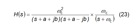
Substituting for a = 0.5, and b = 0.867, and assuming that w_c = 1, from Eq. (23), we obtain

                                                 

4. MODIFYING H(s), WHEN w_c > 1

Equation (20) was derived by assuming w_c = 1. However, in this case, w_c = 151.7 rad/s and we find the pole locations get modified as:

                      Pole B₁ is at (-1) ´ 151.7 = ‒151.7  (25)

           Pole B₂ is at (-0.5+j0.867) ´ 151.7= ‒75.85+j131.376  (26)

          Pole B₃ is at (-0.5-j0.867) ´ 151.7 = ‒75.85‒131.376   (27)

          

Using the above values in Eq. (24), we get

Equation (28) can be simplified to

Equation (29) is used for the design of the analog filter. Table 1 shows the tabulation of the denominator of H(s) with cut-off frequency w_c normalized to 1.